Classification Algorithm : One of Best known method of Supervised Learning

Good morning to all , here is my eleventh blog for you and fourth on the Machine Learning. Today’s topic is Classification Algorithm. Before it we have covered about machine learning and it’s types , Machine Learning real life opportunities and applications and on previous article we have covered regression part of supervised learning. Now today we will see elaborately about Classification algorithm and some of it’s methods used. So here we start :-

We are aware that the algorithms used in supervised machine learning can be generally divided into those used for classification and regression. We have forecasted the results for continuous values using regression techniques, but we require classification algorithms to predict the results for categorical values.

What is the Classification Algorithm?

On the basis of training data, the Classification algorithm is a Supervised Learning technique that is used to categorize new observations. In classification, a program makes use of the dataset or observations that are provided to learn how to categorize fresh observations into various classes or groups. For instance, cat or dog, yes or no, 0 or 1, spam or not spam, etc. Targets, labels, or categories can all be used to describe classes.

In contrast to regression, classification’s output variable is a category rather than a value, such as “Green or Blue,” “fruit or animal,” etc. The Classification algorithm uses labelled input data because it is a supervised learning technique, therefore it comprises input and output information.

In classification algorithm, a discrete output function(y) is mapped to input variable(x).

y=f(x), where y = categorical output

The best example of an ML classification algorithm is Email Spam Detector.

The primary objective of a classification algorithm is to determine the category of a given dataset, and these algorithms are primarily employed to forecast the results for categorical data.

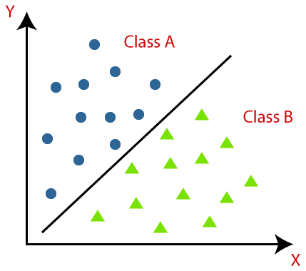
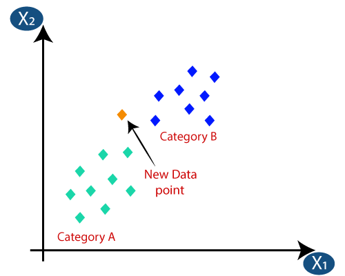
The diagram below can be used to better understand classification methods. There are two classes—Class A and Class B—in the diagram below. These classes share traits with one another and differ from other classes in other ways.

The algorithm which implements the classification on a dataset is known as a classifier. There are two types of Classifications:

• Binary Classifier: If the classification problem has only two possible outcomes, then it is called as Binary Classifier.
  Examples: YES or NO, MALE or FEMALE, SPAM or NOT SPAM, CAT or DOG, etc.
• Multi-class Classifier: If a classification problem has more than two outcomes, then it is called as Multi-class Classifier.
  Example: Classifications of types of crops, Classification of types of music.

Types of ML Classification Algorithms:

Classification Algorithms can be further divided into the Mainly two category:

• Linear Models
  • Logistic Regression
  • Support Vector Machines
• Non-linear Models
  • K-Nearest Neighbours
  • Kernel SVM
  • Naïve Bayes
  • Decision Tree Classification
  • Random Forest Classification

Evaluating a Classification model:

After our model is finished, we must assess its performance to determine whether it is a classification model or a regression model. So, we have the following options for assessing a classification model:

1. Log Loss or Cross-Entropy Loss:

• It is used to assess a classifier’s performance, and the output is a probability value between 0 and 1.
• A successful binary classification model should have a log loss value that is close to 0.
• If the anticipated value differs from the actual value, the value of log loss rises.
• The higher accuracy of the model is shown by the lower log loss.
• For Binary classification, cross-entropy can be calculated as:

?(ylog(p)+(1?y)log(1?p))  ; Where y= Actual output, p= predicted output

2. Confusion Matrix:

• The confusion matrix describes the performance of the model and gives us a matrix or table as an output.
• The error matrix is another name for it.
• The matrix is made up of the results of the forecasts in a condensed manner, together with the total number of right and wrong guesses.
• The matrix appears as the following table:

	Actual Positive	Actual Negative
Predicted Positive	True Positive	False Positive
Predicted Negative	False Negative	True Negative

3. AUC-ROC curve:

• ROC curve stands for Receiver Operating Characteristics Curve and AUC stands for Area Under the Curve.
• It is a graph that displays the classification model’s performance at various thresholds.
• The AUC-ROC Curve is used to show how well the multi-class classification model is performing.
• The TPR and FPR are used to draw the ROC curve, with the True Positive Rate (TPR) on the Y-axis and the FPR (False Positive Rate) on the X-axis.

Use cases of Classification Algorithms

They can be used in different places. Below are some popular use cases :

• Email Spam Detection
• Speech Recognition
• Identifications of Cancer tumor cells.
• Drugs Classification
• Biometric Identification, etc.

K-Nearest Neighbor(KNN) Algorithm

• One of the simplest machine learning algorithms, based on the supervised learning method, is K-Nearest Neighbour.
• The K-NN algorithm makes the assumption that the new case and the existing cases are comparable, and it places the new instance in the category that is most like the existing categories.
• A new data point is classified using the K-NN algorithm based on similarity after all the existing data has been stored. This means that utilizing the K-NN method, fresh data can be quickly and accurately sorted into a suitable category.
• Although the K-NN approach is most frequently employed for classification problems, it can also be utilized for regression.
• K-NN is a non-parametric algorithm, which means it does not make any assumption on underlying data.
• It is also called a lazy learner algorithm because it does not learn from the training set immediately instead it stores the dataset and at the time of classification, it performs an action on the dataset.
• The KNN method simply saves the information during the training phase, and when it receives new data, it categorizes it into a category that is quite similar to the new data.
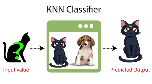
• Example: Let’s say we have a picture of a species that resembles both cats and dogs, but we aren’t sure if it is one or the other. Therefore, since the KNN algorithm is based on a similarity metric, we can utilize it for this identification. Our KNN model will look for similarities between the new data set’s features and those in the photos of cats and dogs, and based on those similarities, it will classify the new data set as either cat- or dog-related.

Why do we need a K-NN Algorithm?

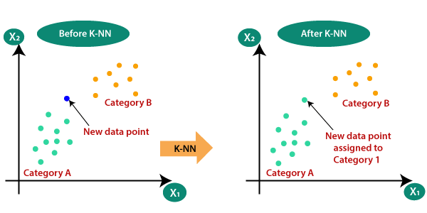
If there are two categories, Category A and Category B, and we have a new data point, x1, which category does this data point belong in? We require a K-NN algorithm to address this kind of issue. K-NN makes it simple to determine the category or class of a given dataset. Take a look at the diagram below:

How does K-NN work?

The K-NN working can be explained on the basis of the below algorithm:

• Step-1: Select the number K of the neighbors
• Step-2: Calculate the Euclidean distance of K number of neighbors
• Step-3: Take the K nearest neighbors as per the calculated Euclidean distance.
• Step-4: Among these k neighbors, count the number of the data points in each category.
• Step-5: Assign the new data points to that category for which the number of the neighbor is maximum.
• Step-6: Our model is ready.

Suppose we have a new data point and we need to put it in the required category. Consider the below image:

• Firstly, we will choose the number of neighbors, so we will choose the k=5.
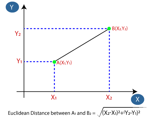
• Next, we will calculate the Euclidean distance between the data points. The Euclidean distance is the distance between two points, which we have already studied in geometry. It can be calculated as:

• By calculating the Euclidean distance we got the nearest neighbors, as three nearest neighbors in category A and two nearest neighbors in category B. Consider the below image:

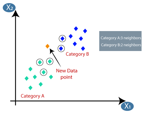
• As we can see the 3 nearest neighbors are from category A, hence this new data point must belong to category A.

How to select the value of K in the K-NN Algorithm?

The following are some things to keep in mind while choosing K’s value in the K-NN algorithm:

• The ideal value for “K” cannot be determined in a specific fashion, thus we must experiment with different values to find the one that works best. K is best represented by the number 5.
• A relatively small number of K, such K=1 or K=2, might be noisy and cause outlier effects in the model.
• Although K should have large values, there may be some issues.

Advantages of KNN Algorithm:

• It is simple to implement.
• It is robust to the noisy training data
• It can be more effective if the training data is large.

Disadvantages of KNN Algorithm:

• Always needs to determine the value of K which may be complex some time.
• The computation cost is high because of calculating the distance between the data points for all the training samples.

Support Vector Machine Algorithm

One of the most well-liked supervised learning algorithms, Support Vector Machine, or SVM, is used to solve Classification and Regression problems. However, it is largely employed in Machine Learning Classification issues.

The SVM algorithm’s objective is to establish the best line or decision boundary that can divide n-dimensional space into classes, allowing us to quickly classify fresh data points in the future. A hyperplane is the name given to this optimal decision boundary.

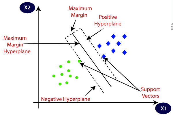
SVM selects the extreme vectors and points that aid in the creation of the hyperplane. Support vectors, which are used to represent these extreme instances, form the basis for the SVM method. Consider the diagram below, where a decision boundary or hyperplane is used to categorise two distinct categories:

SVM algorithm can be used for Face detection, image classification, text categorization, etc.

Types of SVM

SVM can be of two types:

• Linear SVM: Linear SVM is used for linearly separable data, which means if a dataset can be classified into two classes by using a single straight line, then such data is termed as linearly separable data, and classifier is used called as Linear SVM classifier.
• Non-linear SVM: Non-Linear SVM is used for non-linearly separated data, which means if a dataset cannot be classified by using a straight line, then such data is termed as non-linear data and classifier used is called as Non-linear SVM classifier.

Hyperplane and Support Vectors in the SVM algorithm:

Hyperplane Vectors: In n-dimensional space, there may be several lines or decision boundaries used to separate the classes, but we must identify the optimum decision boundary that best aids in classifying the data points. The hyperplane of SVM is a name for this optimal boundary.

The dataset’s features determine the hyperplane’s dimensions, therefore if there are just two features (as in the example image), the hyperplane will be a straight line. Additionally, if there are three features, the hyperplane will only have two dimensions.

We always build a hyperplane with a maximum margin, or the greatest possible separation between the data points.

Support Vectors: Support vectors are the data points or vectors that are closest to the hyperplane and have the greatest influence on where the hyperplane is located. These vectors are called support vectors because they support the hyperplane.

How does SVM works?

Linear SVM:

By presenting an example, the SVM algorithm’s operation can be better understood. Consider a dataset with two tags (green and blue), two features (x1 and x2), and two tags. We need a classifier that can identify whether the pair of coordinates (x1, x2) is blue or green. Think on the photo below:

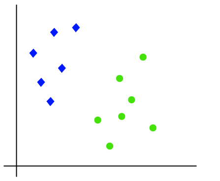
So as it is 2-d space so by just using a straight line, we can easily separate these two classes. But there can be multiple lines that can separate these classes. Consider the below image:

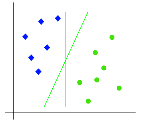
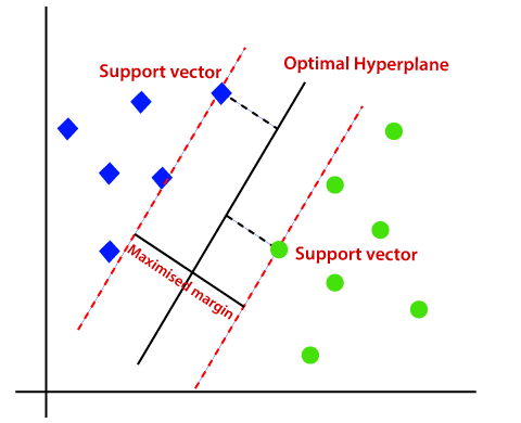
Hence, the SVM algorithm helps to find the best line or decision boundary; this best boundary or region is called as a hyperplane. SVM algorithm finds the closest point of the lines from both the classes. These points are called support vectors. The distance between the vectors and the hyperplane is called as margin. And the goal of SVM is to maximize this margin. The hyperplane with maximum margin is called the optimal hyperplane.

Non-Linear SVM:

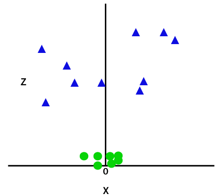
We can use a straight line to divide data that is organized linearly, but we are unable to do so with non-linear data. Think on the photo below:

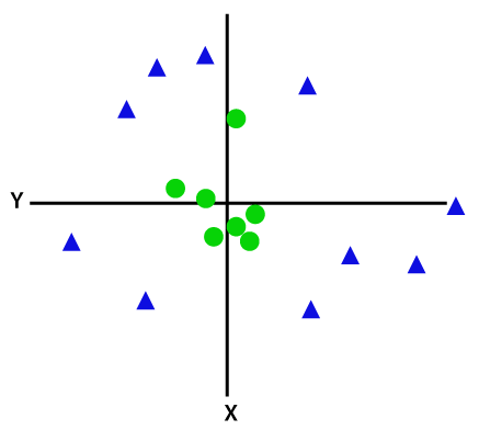
So to separate these data points, we need to add one more dimension. For linear data, we have used two dimensions x and y, so for non-linear data, we will add a third dimension z. It can be calculated as:

z=x2 +y2

By adding the third dimension, the sample space will become as below image:

So now, SVM will divide the datasets into classes in the following way. Consider the below image:

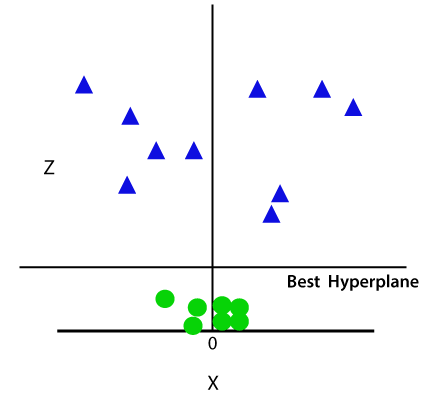
Since we are in 3-d Space, hence it is looking like a plane parallel to the x-axis. If we convert it in 2d space with z=1, then it will become as:

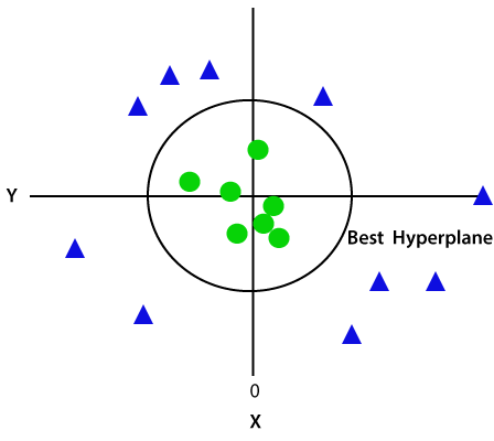
Hence we get a circumference of radius 1 in case of non-linear data.

Naïve Bayes Classification Algorithm

• Naïve Bayes algorithm is a supervised learning algorithm, which is based on Bayes theorem and used for solving classification problems.
• It is mainly used in text classification that includes a high-dimensional training dataset.
• Naïve Bayes Classifier is one of the simple and most effective Classification algorithms which helps in building the fast machine learning models that can make quick predictions.
• It is a probabilistic classifier, which means it predicts on the basis of the probability of an object.
• Some popular examples of Naïve Bayes Algorithm are spam filtration, Sentimental analysis, and classifying articles.

Why is it called Naïve Bayes?

The words Naive and Bayes, which make up the Nave Bayes algorithm, are as follows:

• Naïve: Because it presumes that the occurrence of one trait is unrelated to the occurrence of other features, it is known as naive. A red, spherical, sweet fruit, for instance, is recognised as an apple if the fruit is identified based on its colour, form, and flavour. So, without relying on one another, each characteristic helps to recognize it as an apple.
• Bayes: It is known as Bayes since it is based on the Bayes’ Theorem.

Bayes’ Theorem:

• Bayes’ theorem is also known as Bayes’ Rule or Bayes’ law, which is used to determine the probability of a hypothesis with prior knowledge. It depends on the conditional probability.
• The formula for Bayes’ theorem is given as:

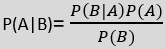
Where,

P(A|B) is Posterior probability: Probability of hypothesis A on the observed event B.

P(B|A) is Likelihood probability: Probability of the evidence given that the probability of a hypothesis is true.

P(A) is Prior Probability: Probability of hypothesis before observing the evidence.

P(B) is Marginal Probability: Probability of Evidence.

Working of Naïve Bayes’ Classifier:

The following example will allow you to understand how the Naive Bayes’ Classifier functions:

Assume that “Play” is the equivalent target variable and that we have a dataset of weather conditions. Therefore, utilizing this dataset, we must determine whether or not to play on a specific day based on the weather. In order to solve this issue, we must take the following actions:

1. Convert the given dataset into frequency tables.
2. Generate Likelihood table by finding the probabilities of given features.
3. Now, use Bayes theorem to calculate the posterior probability.

Problem: If the weather is sunny, then the Player should play or not?

Solution: To solve this, first consider the below dataset:

	Outlook	Play
0	Rainy	Yes
1	Sunny	Yes
2	Overcast	Yes
3	Overcast	Yes
4	Sunny	No
5	Rainy	Yes
6	Sunny	Yes
7	Overcast	Yes
8	Rainy	No
9	Sunny	No
10	Sunny	Yes
11	Rainy	No
12	Overcast	Yes
13	Overcast	Yes

Frequency table for the Weather Conditions:

Weather	Yes	No
Overcast	5	0
Rainy	2	2
Sunny	3	2
Total	10	5

Likelihood table weather condition:

Weather	No	Yes
Overcast	0	5	5/14= 0.35
Rainy	2	2	4/14=0.29
Sunny	2	3	5/14=0.35
All	4/14=0.29	10/14=0.71

Applying Bayes’theorem:

P(Yes|Sunny)= P(Sunny|Yes)*P(Yes)/P(Sunny)

P(Sunny|Yes)= 3/10= 0.3

P(Sunny)= 0.35

P(Yes)=0.71

So P(Yes|Sunny) = 0.3*0.71/0.35= 0.60

P(No|Sunny)= P(Sunny|No)*P(No)/P(Sunny)

P(Sunny|NO)= 2/4=0.5

P(No)= 0.29

P(Sunny)= 0.35

So P(No|Sunny)= 0.5*0.29/0.35 = 0.41

So as we can see from the above calculation that P(Yes|Sunny)>P(No|Sunny)

Hence on a Sunny day, Player can play the game.

Advantages of Naïve Bayes Classifier:

• One of the quick and simple machine learning techniques to predict a class of datasets is naive Bayes.
• Both binary and multi-class classifications can be done with it.
• In comparison to other algorithms, it performs well in multi-class predictions.
• It is the most frequently used solution for text classification issues.

Disadvantages of Naïve Bayes Classifier:

• Naive Bayes assumes that all features are independent or unrelated, so it cannot learn the relationship between features.

Applications of Naïve Bayes Classifier:

• It is used for Credit Scoring.
• It is used in medical data classification.
• It can be used in real-time predictions because Naïve Bayes Classifier is an eager learner.
• It is used in Text classification such as Spam filtering and Sentiment analysis.

Types of Naïve Bayes Model:

There are three types of Naive Bayes Model, which are given below:

• Gaussian: The Gaussian model assumes that features follow a normal distribution. This means if predictors take continuous values instead of discrete, then the model assumes that these values are sampled from the Gaussian distribution.
• Multinomial: The Multinomial Naïve Bayes classifier is used when the data is multinomial distributed. It is primarily used for document classification problems, it means a particular document belongs to which category such as Sports, Politics, education, etc.
  The classifier uses the frequency of words for the predictors.
• Bernoulli: The Bernoulli classifier works similar to the Multinomial classifier, but the predictor variables are the independent Booleans variables. Such as if a particular word is present or not in a document. This model is also famous for document classification tasks.

Conclusion

Today we have covered classification and regression was covered in previous article. Here we come to know about classification algorithm and about various types of algorithms used for classification, how they work and many more. For more blogs like this visit our website : Theax Blogs .